Step 3- Spectral analysis

In this step of the tutorial we will see how to obtain an average H/V spectral ratio curve that is sufficiently representative of the recording.

You can load the file "Step_2" inside the tutorial folder, which contains the data needed to proceed from this point of the tutorial onwards.

1. First of all click on the Tab named "Spectral analysis" as shown in the following figure

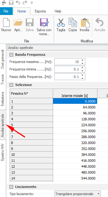
1. We define the frequency band to be analysed by setting the values in the section named "Frequency band". We set the minimum frequency value to 0.1 Hz, and the step to 0.1 Hz as shown in the image below

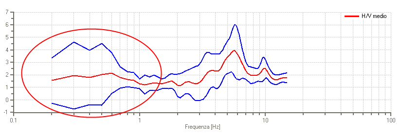
1. In the right-hand part of the application window the charts will also have changed. In particular the H/V spectral ratio chart will look like this:

1. The red ellipse in the previous image outlines an area of the average H/V spectral ratio with an excessive standard deviation, represented by the blue curves. In order to obtain a good result, the width of the space between the two blue standard deviation curves must be reduced. To do this we can exploit the stationarity map, which allows us to identify those spectra with strong components at the frequencies where the standard deviation is excessive, since the stationarity map collects all the spectral ratios of each window selected in the previous stage of the analysis.

2. Before discarding the windows that generate an excessive standard deviation, it is possible to change the type of smoothing applied to the spectral curves. In the section named "Smoothing" several options are available. For the purposes of the tutorial only, we set the smoothing type according to Konno & Ohmachi as in the following figure

Pressing the "Update" button gives the following spectral ratio chart:

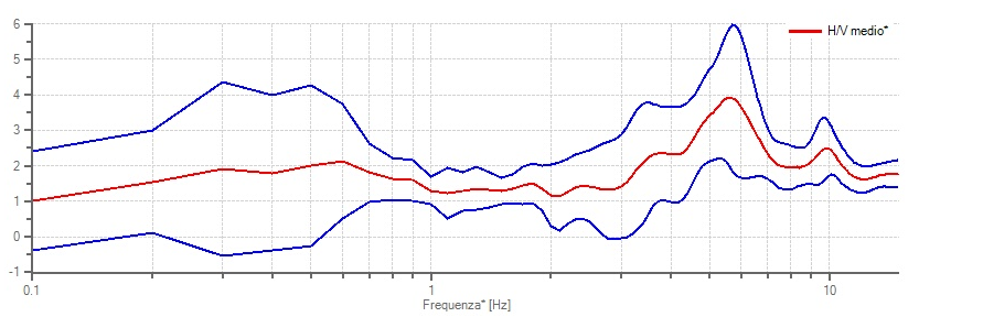
From the image above it can be seen how changing the type of smoothing affects the shape of the average spectral ratio curve and of its standard deviation, while leaving its content unchanged. In fact the peak of the curve remains at practically the same frequency.

For further information on the types of smoothing and their parameters, see the relevant section of this manual.

1. We now set the smoothing type back to "Proportional triangular", leaving the smoothing percentage at 10 %, and press update to return to the previous conditions.

2. We now change the type of directional sum, from "arithmetic mean" to "geometric mean" as shown in the following figure

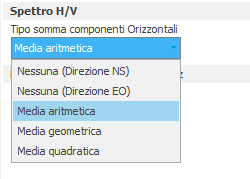
1. Pressing the "Update" button, the average H/V spectral ratio chart changes and takes the following form:

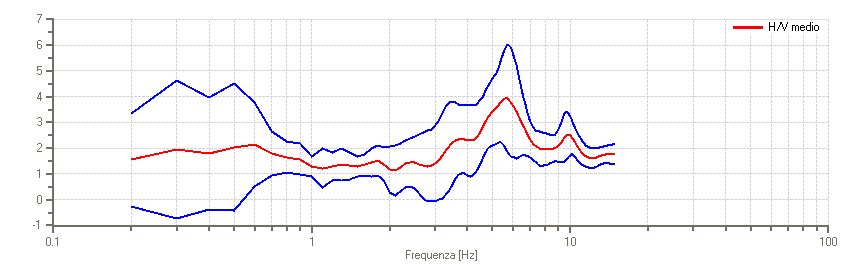
It can be noted that in this case the substantial difference lies in the increase of the ordinates of the curve. For further details on the types of directional sum, see the relevant section of this manual.

1. Let us now look at the stationarity map:

This map provides useful information for identifying which windows should be excluded from the analysis. In the image above the spectra of those windows with a large component at the frequencies where the standard deviation is high have been highlighted. These windows can be recognised by the fact that they show red and yellow "small squares" at those frequencies. To exclude such windows you can click on the map at those "small squares". This selects the corresponding window within the table of the "Selection" section

1. By clearing the check mark in the "Selected" column of the row associated with the spectrum to be excluded and pressing "Update", that window will not be considered in the generation of the H/V spectral ratio curve. Repeating the operation for all the windows highlighted in the previous stationarity map gives the following result:

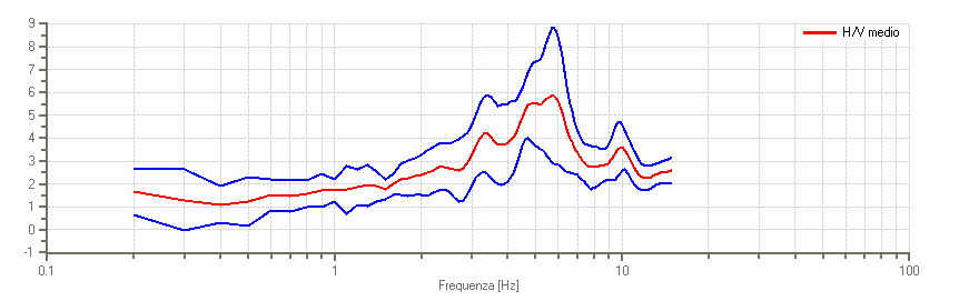
As can clearly be seen, the width of the corridor identified by the two blue standard deviation curves highlighted in the previous images has decreased appreciably. The spectral ratio obtained in this way can therefore be considered valid, that is representative of the recording.

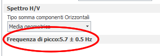
1. In the lower left part of the application window you can read the frequency at which the peak of the average H/V spectral ratio curve is located, together with its uncertainty, as in the figure below:

©Geostru