Local seismic response analysis
Before performing a local seismic response analysis, it is possible to define a set of monitored nodes, at which the analysis results will be returned. The advantage of assigning monitored nodes lies in a considerable reduction of the computation time, since the local seismic response will be returned only with reference to those nodes and not for the whole domain. To select a monitored node, in the Tools panel, after selecting the node, simply click on the "Add monitored nodes" button in the top bar.

The monitored nodes are highlighted as shown in the figure above.
To perform the local seismic response analysis, use the "Seismic response analysis" button in the Analysis and results panel. This command opens the window shown below.

In this window it is possible to select different analysis options, including:
a) Without rigid displacements
b) Relative displacements and velocities
Option (a) does not consider, in the dynamic analysis, the absolute rigid displacement of the system. This option should generally be selected, since rigid displacements do not entail additional stresses.
By selecting option (b), at the end of the calculation the relative displacement is returned for each node; otherwise the displacement returned is the absolute one.
Seismic analysis data
The RSL III 2D software allows four types of analysis to be performed:
- Equivalent nonlinear analysis
- Linear analysis with variable damping
- Linear analysis with constant damping
- Dynamic analysis

Types of analysis available in RSL III 2D
From a theoretical point of view, the dynamic analysis for a finite number of nodes is performed by solving a system of equations of the type:

where
[M] = mass matrix
[C] = damping matrix
[K] = stiffness matrix
R = vector of the known loads, equal to [M]ag, with ag the input accelerogram.
u is the vector of the relative displacements.
The system is solved in the time domain according to Newmark's criterion: it consists of a series of successive integrations, for each step Δt, that allows the velocity and, therefore, the relative displacement u to be determined. In the application of Newmark's method some integration parameters are required (red box in the following figure).

Beta and Gamma are two parameters of the Newmark integration method which generally have a value of 0.25 and 0.5, respectively.
The soil damping is taken into account through the matrix [C]. For each element i into which the domain is subdivided, Ci is computed according to Rayleigh's criterion, which is related to mass and stiffness:
Ci = α∙Mi + β∙Ki
where α and β are two coefficients called, respectively, Rayleigh mass and Rayleigh stiffness, while Mi and Ki are the mass and stiffness of the single element. Using this formulation, the damping λ (or damping ratio) can be made dependent on the circular frequency according to the following relationship:
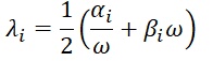
where α and β for the i-th element are computed as follows:

with w1 the main frequency corresponding to the first mode of vibration.
Linear analysis with constant damping (red box in the figure below): the software performs the calculation using the consistent Rayleigh damping matrix, with α and β constant for all the nodes and equal to the values indicated in Rayleigh Mass and Rayleigh Stiffness.
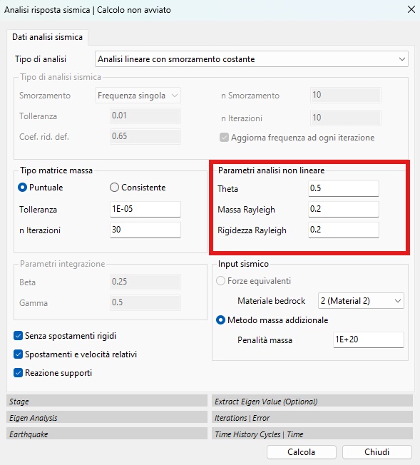
Theta is an integration parameter generally set equal to 0.5.
Linear analysis with variable damping: the software performs the calculation using, as damping parameters, those defined in the materials grid.
Equivalent nonlinear analysis (red box in the following image).
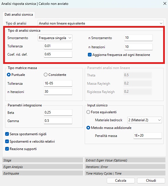
In this case the software performs a sequence of linear analyses in which the stiffness and damping parameters are updated iteratively until a convergence factor is reached. The calculation starts with the initial values of G and D entered in the materials window, and the shear strain associated with the displacement value u is determined. In each iteration the values of D and G/Gmax are updated as a function of the effective strain level reached, and the calculation stops when the difference of the G and D values between one iteration and the next is lower than the tolerance level set by the user.
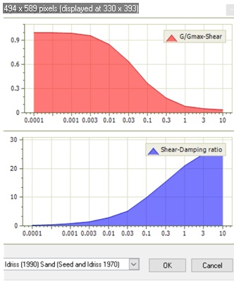
For this type of analysis it is also possible to choose to update the circular frequency w at each iteration. This implies that the computation of the Rayleigh coefficients α and β in the damping matrix C is updated at each iteration for each element, as a function of the main frequency w1, in the case of Single frequency, or of w1 and w2 in the case of Double frequency. For each element, in the case of Double frequency, the expressions of α and β are:
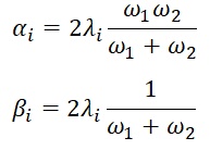
with w1 the main frequency and w2 = nDamp × w1, where nDamp is generally set equal to 10. In essence, for each iteration the mean shear strain is computed for each element, and the damping curve is consulted to update the correct value of the damping.
The Tolerance defines the difference between the values of G and D, found between one iteration and the next, which determines the end of the iterative calculation.
The No. of iterations establishes how many iterations must be performed by the program: a high number of iterations (>10) entails a useless increase of the computation time.
Strain red. coeff. is a coefficient that reduces the maximum strain; its value is usually set equal to 0.65. It is computed from the following expression: γeff/γmax = (M − 1)/10.
Other parameters of the equivalent nonlinear analysis concern the finite element modal analysis, in which the mass matrix must be defined (red box):

Lumped mass: the mass is considered concentrated at the nodes.

In this case the structure of the mass matrix is diagonal and entails considerable advantages, due to the lower memory usage and the substantial reduction of the computation time. Usually this assumption does not entail large errors and is therefore preferable.
Consistent mass: the mass is distributed and the corresponding matrix is essentially full and symmetric. This assumption produces smaller errors in absolute value, but entails an increase in the computation time.
Modal analysis parameters: for the modal analysis, a Tolerance factor must be set, which establishes when the calculation must stop, together with a No. of iterations. If the calculation reaches the set number of iterations, it stops even if the desired tolerance has not been reached. The modal analysis must be performed for all the nodes of the domain, and is therefore not carried out by the software when monitored nodes are present.
Seismic input
In the execution of the RSL III 2D calculation, it is possible to choose two different methodologies: Equivalent forces and Additional-mass method.
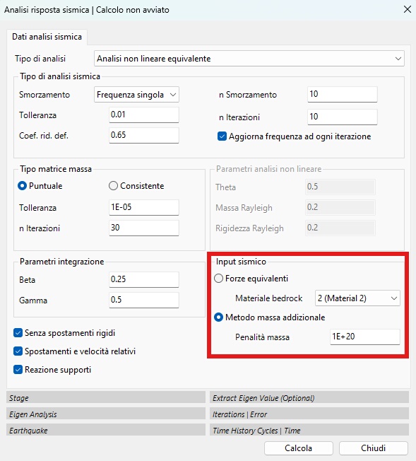
With the first approach, the seismic input is defined in terms of equivalent nodal forces (or effective seismic forces), which are proportional to the velocity of the incident wave and are applied in the horizontal direction along the base of the domain defined by the model. This type of seismic input (outcrop input) is considered as a time-dependent shear force:
F(t) = ρVsAv(t)
where ρ is the density of the bedrock, Vs represents the velocity of the S waves in the bedrock, v(t) represents the velocity of the earthquake and A represents the tributary area associated with the loaded node.
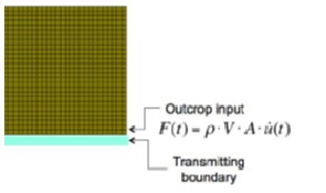
Seismic input, equivalent-forces approach
These forces are computed automatically by the software and are applied at the nodes of the domain in contact with the bedrock; the advantage of this method is therefore precisely that of not having to model the bedrock layer, but only having to choose the material it is made of. By selecting this method, the boundary conditions in Phase 1 are represented by springs, both horizontal and vertical, for all the boundary nodes of the domain. In Phase 2 the software automatically computes the reactions of the springs for all the domain boundaries.