Seismic piezocone (SCPTU)¶

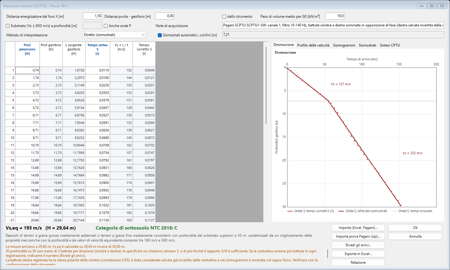
The Seismic piezocone (SCPTU) window (test menu, Seismic piezocone (SCPTU)..., or Import readings → Seismic SCPTU test) holds the seismic part of the test: S (and P) wave arrival times, interpretation, velocities, Vs,eq and ground type according to the Italian NTC 2018. The piezocone readings (qc, fs, u2) stay in the same test and are also used for the CPTU summary chart.

SCPTU window

Data sources¶

Pagani acquisition unit records (Import Pagani test (zip)...): the zip or folder of the test, with one subfolder per depth containing the GSL (left) and GSR (right) shots for S waves and, if present, GSN (vertical shot) for P waves. The unit records traces, not times: the program filters the signals, picks the arrival times and shows them on the seismograms for checking (see Picking). Several files of the same direction in one folder are several shots: they are stacked and counted.
Field sheet (Import (Excel, Pagani)...): .xlsx, .xls or .csv with depths and arrival times already read with another program. Headers, source offset (Offset row), tip-geophone distance and acquisition notes are recognised.
By hand or pasting from Excel: input columns Cone depth, S arrival time, P arrival time.

Piezocone readings (qc, fs, u2) are imported with Import readings → Pagani TGAS (XML, Excel): besides the TGAS XML, the Excel sheet exported by the unit is read as well (row Depth, Qc, Fs, U2, ..., depths in cm), including the water table (Hydrostatic Line). To keep CPTU and seismic data in the same test, import the file from the test readings window.

Parameters¶

Parameter	Meaning
Source distance from the hole X	horizontal distance between the source plate and the rods. It is not in the Pagani files: enter it.
Tip - geophone distance	geophone depth = tip depth − this distance. 0 for Pagani files (their depths are already geophone depths).
Average unit weight	for G0 = ρ·Vs².
Bedrock	depth of the bedrock (Vs ≥ 800 m/s) if within 30 m: H of Vs,eq.
Interpretation method	Direct (seismic layers) or Pseudo-interval.
Automatic seismic layers, boundaries	layer boundaries of the direct method, found by the program or entered by hand (e.g. `7.2; 16.5`).

Picking the arrival times¶

S-wave picking

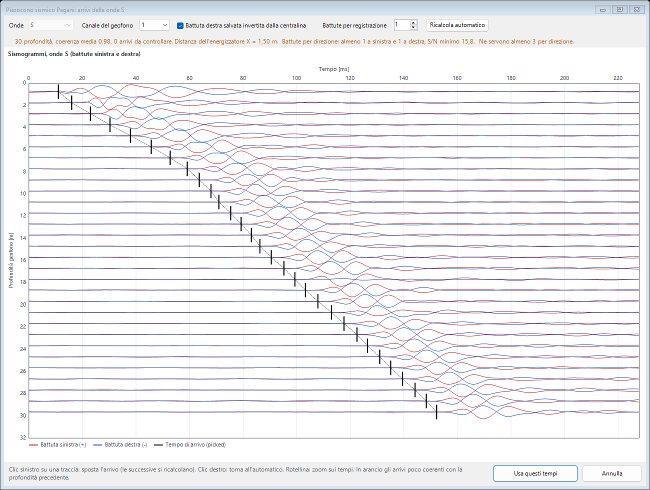
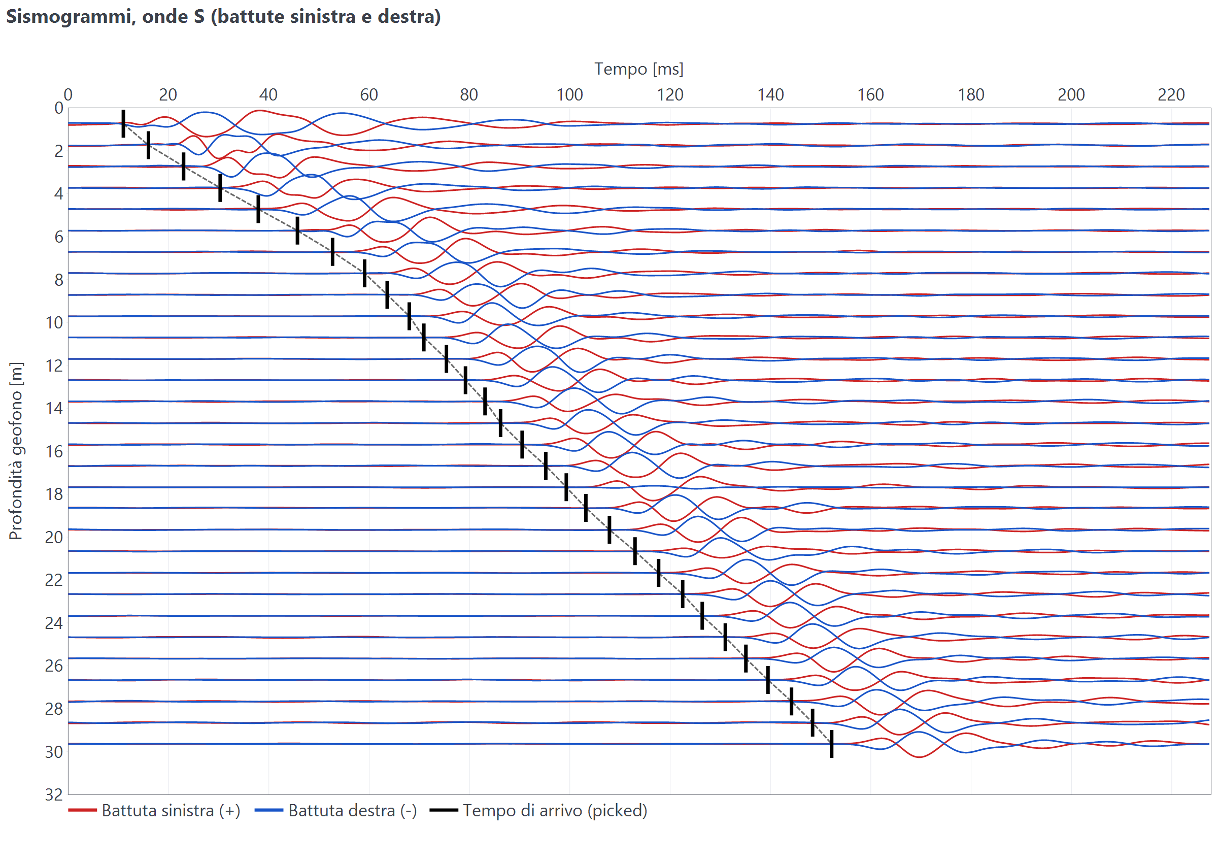
At each depth the left shot (red, +) and the right shot (blue, −) are overlaid: reversing the blow reverses the signal, so the two traces are in phase opposition and the S-wave first arrival is where they separate. The black mark is the chosen arrival time; the dashed line joins the arrivals.

Zero-phase band-pass filter 10-140 Hz (P waves: 20-400 Hz).
Geophone channel with the highest coherence between adjacent depths (can be changed).
First arrival at the first depth, then times by waveform correlation with the previous depth; poorly coherent arrivals in orange.
Left click on a trace moves the arrival (following depths are recomputed), right click returns to automatic, mouse wheel zooms the time axis. With Waves: P the P arrivals are checked in the same way.
Right shot saved inverted by the acquisition unit: some units save the right shot already inverted. The program detects it from the correlation between the two recorded shots and always shows the right shot with its physical sign; the choice can be changed.
Shots per record: if the unit stacks several blows in each record, enter their number. Above the seismograms the number of shots per direction and the minimum signal-to-noise ratio (S/N) are shown; below 3 shots per direction a warning appears (many specifications require at least 3, or more until S/N is sufficient).

The stacked traces are saved in the test: Review arrivals... reopens the seismograms without the original files.

Interpretation methods¶

Geophone depth z = tip depth − tip/geophone distance, source-geophone path L = √(z² + X²).

Direct method (seismic layers)¶

This is the method to use with a single receiver (the differential method is valid with two receivers). Each time is reduced to the vertical, tc = t·z/L, and on the corrected time - depth diagram (travel-time curve) the seismic layers with constant velocity are identified. In each layer the least-squares line tc = t0 + z/V gives the layer velocity (Vs with S waves, Vp with P waves), with its R².

Seismic layers

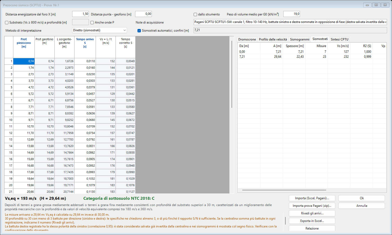
With Automatic seismic layers the boundaries are found by splitting the travel-time curve into straight segments of at least 3 readings; the number of segments is chosen with the BIC criterion, taking the picking precision as minimum noise. Unticking it, boundaries are entered by hand, starting from the ones found.

Pseudo-interval¶

As in field sheets: interval velocity Vs = (L2 − L1)/(t2 − t1) between successive readings, starting from z = 0, L = 0, t = 0.

Results¶

Vs,eq = H / Σ(hᵢ/Vsᵢ) (NTC 2018, §3.2.2), H = bedrock depth if within 30 m, otherwise 30 m; ground type with the description of table 3.2.II.
G0 = ρ·Vs² and, with P waves, Poisson's ratio and E0 = 2·G0·(1 + ν).
Tabs Travel-time curves, Velocity profile, Seismograms, Seismic layers, CPTU summary. Right click on a chart: copy or save the image.
Export to Excel...: table with the columns of the chosen method and the results.

Report¶

The test report contains: CPTU summary chart, parameters and acquisition notes, method description, arrival time table (measured and corrected, shots per direction, S/N), seismic layer table, Vs,eq and ground type, warnings, stacked seismograms of S waves with the two shots in two colours and the picked times (and of P waves, if present), travel-time curves and velocity profile.

Seismograms in the report

CPTU summary chart¶

CPTU summary

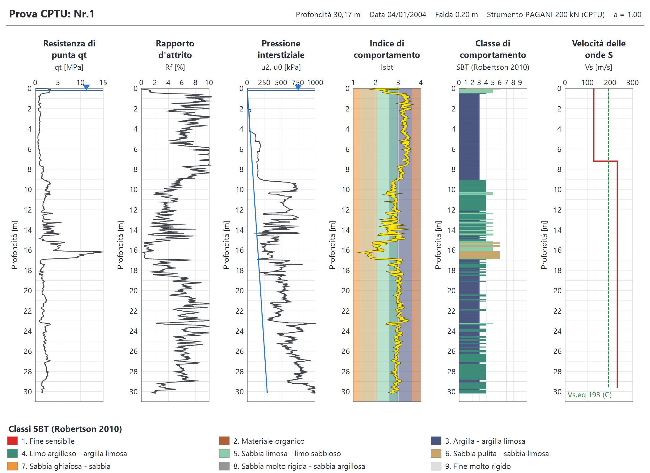
For piezocone tests (u2 readings) the program draws a one-page summary: corrected cone resistance qt = qc + u2·(1 − a), friction ratio Rf = fs/qt, pore pressure u2 with the hydrostatic line u0 from the water table, behaviour index Isbt over the class bands and the SBT class column (non-normalized chart by Robertson, 2010, 9 classes); with the seismic test, also the Vs profile with Vs,eq. The area ratio a is taken from the instrument (0.80 if not set).

Isbt = √[(3.47 − log(qt/pa))² + (log Rf + 1.22)²], pa = 100 kPa; classes 2-7 from the limits 3.60 - 2.95 - 2.60 - 2.05 - 1.31, classes 1, 8 and 9 from the zones of the qt/pa - Rf chart.

References¶

Butcher A.P., Campanella R.G., Kaynia A.M., Massarsch K.R. (2005). Seismic cone downhole procedure to measure shear wave velocity - a guideline. ISSMGE TC10.
ASTM D7400. Standard Test Methods for Downhole Seismic Testing.
Robertson P.K. (2010). Soil behaviour type from the CPT: an update. 2nd International Symposium on Cone Penetration Testing, Huntington Beach.
NTC 2018, §3.2.2 and table 3.2.II.

©Geostru