Data interpretation
Objective of this step: to move from the traveltime curves to the subsoil section — depth and shape of the refractors, velocity and elastic parameters of the layers. The software applies Palmer's (1980) Generalized Reciprocal Method (G.R.M.).
In the Interpretation section you will find four tabs, to be worked through in order: Velocity function, Time-depth function, Morphology of refractors and Velocity map.
1. Velocity function → optimum XY
The velocity function serves to determine the true velocity of the refractor. The software proposes several curves, one for each trial value of the XY parameter.
Which curve to choose
Choose the curve that shows the lowest degree of irregularity, that is the straightest trend. The curve selected defines the optimum XY value, which will be used in all the subsequent stages of the G.R.M. processing.
This is the parameter introduced by Palmer in order to reconstruct irregular refractors, whereas the earlier methods (reciprocal shooting, delay time, plus–minus) assumed surfaces of gentle and regular dip.
2. Time-depth function
Once the optimum XY has been calculated, the software builds the time-depth curve, which considers depth instead of the inter-geophone distance. This curve has a precise physical meaning: it returns the shape of the refracting horizon expressed in the time domain, that is the trend of the refractor before conversion into metres.

3. Morphology of the refractors
This is the actual result: the 2D section of the subsoil.
Geometrically, the projection of each geophone onto the discontinuity is treated as the radius of a circle; the refractor is reconstructed as the envelope of tangents to the circular arcs drawn beneath all the geophones.
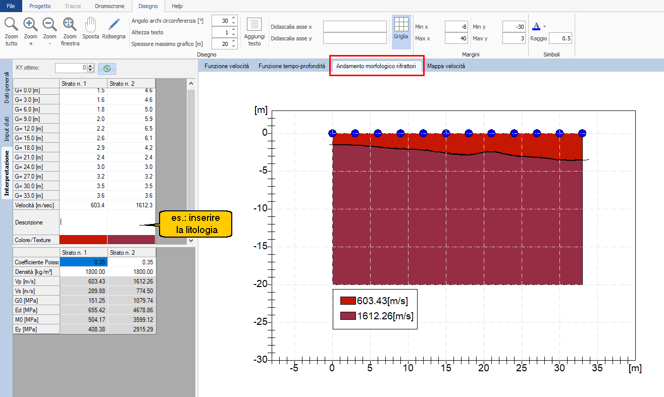
From the Drawing menu you can adjust the graphical rendering: angle of the circular arcs, layer thickness, horizontal extent of the section, colour and radius of the geophone symbols; you can also insert texts (survey title, locality, date) and zoom.
Closer geophone spacing, more faithful refractor
The level of detail with which the surface is reconstructed depends on the density of the geophones: small spacings return a more articulated refractor, closer to reality.
4. The numerical results
Alongside the section, the grid gives for each layer the depth beneath each geophone and the calculated parameters:
| Quantity | Meaning |
|---|---|
| Vp | velocity of the compressional waves |
| Vs | velocity of the shear waves |
| G0 | shear modulus at small strains |
| Ed | dynamic modulus |
| M0 | oedometric modulus |
| Ey | Young's modulus |
| Poisson's ratio, Density | values assigned per layer |
By clicking on a value the software shows its extended description. In the Description field you can assign a lithological name to each layer (e.g. weathered layer, fractured schists), which will appear in the section legend and in the report.
Velocity does not identify the lithology
Assign the lithological names with caution and, where possible, calibrate them against a borehole. Within the same material velocity varies with compaction, fracturing and porosity: two layers with different velocities may be the same lithotype under different conditions.
5. Velocity map
The last tab returns the distribution of velocities in the subsoil as a colour map: cool colours = low velocities, warm colours = high velocities. It is an overall reading that is useful for quickly identifying lateral anomalies.

If the result does not add up, go back to the picking
The morphology of the refractors depends directly on the first arrivals. If the section shows implausible shapes or abrupt steps, the cause is almost always a first arrival read badly on one or two traces. Go back to Data input → Traces, correct the picking with the zoom window and recalculate: the section is updated accordingly.
6. Generating the report
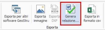
Once the study is complete, click on Generate report. The report automatically collects general data and study area, tables of geophone position and elevation, first arrivals, traveltime curves, refractors, velocity and time-depth diagrams, stratigraphic section and elastic parameters, as well as theoretical notes and the formulas of the method.
What you see is what you print
The diagrams go into the report exactly as they are set at the moment of generation: if in the Traveltime curves tab you have left only the direct ones selected, only those will appear in the report. Before generating, set the views you want to document (normally Shots: all, Traveltime curves: all).
The report can be exported in RTF, DOC, DOCX, PDF and HTML; from the Project bar you can also export the image of the section, the DXF, a CSV file and the data for other GeoStru software.
Before you deliver, it is worth going through the Quality checks and common mistakes.